Organizing Geospatial data with Spatio Temporal Assets Catalogs — STAC using python
- Mauricio Cordeiro
- Mar 12, 2023
- 6 min read
How to create a STAC catalog for geospatial data in Python with the pystac package

Introduction
Those who work with geospatial data may be used to the huge amounts of files to deal with. Normally plenty of steps with intermediate files have to be processed to achieve the final goal. Besides that, with the increasing availability of free satellite imagery with higher spatial resolution and the advance in computational power, larger areas of interest are being object of study and even more files are needed to cover everything.
Geospatial clouds such as the Google Earth Engine and the Microsoft Planetary Computer are great options to avoid all the hassle of dealing with single files (some stories about them here and here), but sometimes it is inevitable to process them locally.
In a recent project, to assess water surface extents from 2018 to 2021 in south east of Brazil, I had to cover an area of approximately 320,000km² using Sentinel-2 imagery in full spatial resolution (10m). 20m bands have been upscaled accordingly. Surface water masks for each image were created using a modified version of the waterdetect package (read more about it in the story: Water Detection in High Resolution Satellite Images using the waterdetect python package).
To cover the whole region of interest of the study, a total of 36 tiles have been selected. Considering the time frame, approximately 12,000 files have been individually processed.

To organize all the work I’ve used STAC catalogs locally, in Python, and I will demonstrate how to create a STAC catalog and then how to quickly access portions of it (and stacking assets) using client packages such as stackstac.
Why STAC catalogs
Intermediate products have been created for each one of 12,000 files, as well as individual reports and other scatter plots for quality assessment. To process all these files, people usually rely on filenames (or folder names) to link the intermediate works, but that’s prone to errors.
Moreover, simple tasks such as querying the images that cover a specific region are not feasible just with the filenames. Besides that, each image can have different properties such as shape and spatial projection, so it is not straightforward to compare them without having more underlying information. And that’s exactly where STAC catalogs fits in. According to their official page https://stacspec.org/:
The SpatioTemporal Asset Catalog (STAC) specification provides a common language to describe a range of geospatial information, so it can more easily be indexed and discovered. A ‘spatiotemporal asset’ is any file that represents information about the earth captured in a certain space and time.
In a nutshell, it is a standard XML specification to describe the geospatial image (or any other asset, such as a PNG thumbnail, for example). And these specifications are organized in a structure of catalogs, sub catalogs and collections (Figure 2). Each STAC item has a reference (link) to the place of the assets, whether they are stored in a filesystem or hosted in the cloud. This way, once your catalog is created, it doesn’t matter where exactly are the files, and you can perform searches by region, or by date, just looking at the catalog items.

Many satellite imagery providers are publishing their datasets following the STAC specification (Figure 3) but for local catalogs it is not so common and I found very little information about it and how to create a STAC catalog in python, for example.

Creating a STAC catalog
Now I will show you how to create a STAC catalog in Python, using the pystac package. First thing is to have some images to catalog. I will select a subset of my Sentinel-2 water masks, but the code should work similarly for any geospatial imagery that is accepted by xarray. I separated the files by TILE and each date has 3 different files as shown in Figure 4:
1- the water mask itself (.tif);
2- a quick view (thumbnail.png); and
3- the output scatter graph (graph.png).

The packages that we will need are:
rasterio
shapely
pystac
stackstac
The code snippet to create the basic catalog is rather simple. Pay attention to the stac_extensions argument. It will be needed in the following steps to add projection properties to the asset (more explanations on Create Assets section).
Creating STAC Items
To create the items, we will loop through our files. Each item will have 3 assets associated (watermask, thumbs and graphs).
One advantage of using a geospatial catalog, as mentioned in the Introduction, is that it will allows us to search data by datetime or location without actually opening each image or parsing the name string. For this, our items will must have some properties such as Geometry, Bounding Box, Datetime, etc. To extract the geospatial information from our masks (the other 2 assets are not “geospatial”) we will create the following function. It will work with datasets opened with rasterio or xarray (as long as rioxarray package is also installed)
Now we will create the items. Note that we will project the bounding box and footprint to WGS84 (epsg:4326) before writing the properties to the item. If you are not used to Coordinate Reference Systems (CRS) I’ve written a tutorial about it in my Python for Geosciences series here on GeoCorner: Python for Geosciences: Raster Merging, Clipping and Reprojection with Rasterio
We also need to give the item an ID, a datetime and optionally, we will write the TILE code. We will get all of them from the Path object. The describe function at the end gives us a summary of the catalog:
2331
* <Catalog id=Paranapanema>
     * <Item id=S2A_MSIL2A_20180103T133221_R081_T22KDV>
     * <Item id=S2A_MSIL2A_20180116T134201_R124_T22KDV>
     * <Item id=S2A_MSIL2A_20180123T133221_R081_T22KDV>
     * <Item id=S2A_MSIL2A_20180215T134211_R124_T22KDV>
     * <Item id=S2A_MSIL2A_20180222T133221_R081_T22KDV>
     * <Item id=S2A_MSIL2A_20180225T134211_R124_T22KDV>
Et voilà. We’ve added 2331 items to our catalog. But it is still missing the path to each asset. We will add them in the next step.
Create Assets
Note that we now have a catalog with items, but we don’t have the path to the actual files anymore. For educational purposes I separated it in 2 steps (create items and create assets) but in “real-life” you should consider writing everything in the same loop. Now we will have to loop through the items again and get the correct item from the ID to add the assets to it.
Besides that, we will need the bounding box and footprint again, but we will leave them in the original CRS. That will make it easier to open these assets with stackstac in the future.
To add the projection information to the asset we will need to use an Stac Extension called Projection Extension. The Project Extension provides a way to describe Items whose assets are in a geospatial projection. It will add a list of properties to the asset (check its manual for a full list) but we will use the following:
proj:epsg,
proj:geometry,
proj:bbox,
proj:shape,
proj:transform.
To use a STAC Extension in a Catalog it must be defined during the creation of the catalog. That’s why we added the extension to the catalog and to the item. So, here is the code to add the water mask asset to our items:
Create Media Assets
To create media assets is much simpler. Again, we will loop through our files, but there is no need to get the geospatial properties.
If we would like to check if the assets have been created correctly, we can access the item property assets, like so:
item.assets
{'watermask': <Asset href=paranapanema/22KGV/S2B_MSIL2A_20210817T132229_R038_T22KGV_watermask.tif>,  'thumbnails': <Asset href=paranapanema/22KGV/S2B_MSIL2A_20210817T132229_R038_T22KGV_thumbs.png>,  'graphs': <Asset href=paranapanema/22KGV/S2B_MSIL2A_20210817T132229_R038_T22KGV_Graphs.png>}
Saving
Before saving, it is important to understand that each item will have a .json file written to disk. in which folder will depend on the “strategy” that we haven’t set yet. The default is a subfolder for each item id, under the root catalog folder. We will leave it default.
To create the hrefs, we need to use .normalize_hrefs and pass the root folder.
Testing
To test our catalog, let’s open it in a new variable and display one item as dictionary to see the results.
To finish, let’s see it in action with stackstac. First we will create a function to select items by tile and by datetime and grab the items in one specific month.
In my example, it returned 19 items. Now let’s combine them using stackstac and create a nice mosaic for displaying. Note that we don’t have to bother with CRSs and projections, as these information are already saved in the asset.
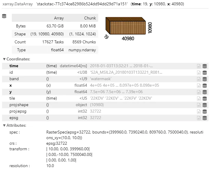
As you can see, it created a “lazy” data cube with our 19 images and we will now perform the median computation to create a month layer.

Conclusion
I will leave you with this beautiful water surface mosaic from the Paranapanema basin, Brazil.
Today we’ve learnt a little about STAC catalogs and how to use them to organize geospatial data. As you could see in the Testing section, once we have our catalog well “organized” it is much easier for future operations and analysis. And that’s really important given the amount of files and processing steps needed for geospatial analysis.
I hope you have enjoyed this tutorial. And see you in the next story!
Hello,
Firslty, I would like to thank to you for this great tutorial.
However, I having a trouble, because when I check the catalog.describe(), I got 0 besides 2331 in your case. What might be the reason of it? (I followed exactly same steps as you did)
Thanks in advance.