Python for Geosciences: Raster bit masks explained (step by step)
- Mauricio Cordeiro
- Mar 28, 2022
- 11 min read
Learn how to (correctly) use raster bit masks layers provided by satellite images as quality assessment bands

Introduction
Welcome back to the 4th part of the Python for Geosciences series. In the previous post we have covered how to extract the bands values to proceed a simple spectral analysis. Imagine, however, that our final objective is to automatically monitor the reflectance spectra of a specific area of interest. This could be a crop, a forest, a lake or any other target and the goal is to check the evolution of the spectral reflectance of this area over the time (this can be used, for example, to identify a specific type of crop, monitor the evolution of a water parameter, etc.). This task could be easily automated (we will see automation in the next post), but there is an issue we should take care of if we want to run this kind of monitoring in the “auto-pilot” mode. Undesired pixels such as clouds and shadows can block the view of the satellite sensor and cause noise in the data or the pixels can be defective for any other kind of interference. That’s where the satellite Quality Assessment layers (and masking) comes in. For those not familiarized with this topic, the images acquired by the satellite sensors have to be corrected for atmospheric interference, solar angle, and other effects before we can use it as a surface reflectance (also called BOA — Bottom of Atmosphere reflectance). More details on this subject can be found in the chapter “The Atmospheric Correction Problem” from the Ocean Optics Web Book [1], available here.
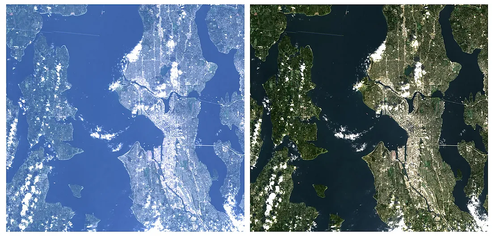
Figure 1 shows a comparison of a Top of Atmosphere (TOA) reflectance composite using bands 4, 3, 2 (natural color composition) and a Surface Reflectance (SR) composite using the same bands, processed using the Land Surface Reflectance Code (LaSRC) processor for Landsat 8.
Each satellite mission has its own atmospheric correction processor but other processors can also developed by researchers and institutions for specific applications. As an example of this diversity, Sola et. al. assessed four different atmospheric correction methods developed specifically for the Sentinel 2 images in the article “Assessment of atmospheric correction methods for Sentinel-2 images in Mediterranean landscape” [2].
The good news is that during this step, that is responsible for bringing an satellite image from the Level 1 (Top of Atmosphere) to Level 2 (Surface Reflectance) of processing, most of these processors classifies the pixels according to its composition (cloud, water, land, et.), and also identifies problematic pixels that should be avoided such as high saturated pixels, and others. The bad news is that there is no standardization and each processor applies its own logic for the processing and for the output products. In this scenario, it is important that we fully understand the product we are working with but also that we have the foundations to be able to deal with any of these cases, and that’s our objective today.
Step 1- Landsat Quality Assurance Bands
The first step is to understand the product we are working with (in our case, the Landsat 8 image from the Amazon region). For this, we have to correctly identify our product. Let’s take a look at it’s name:
LC08_L2SP_231062_20201026_20201106_02_T1Ok. But what those letters and numbers really mean? If we refer to the naming convention for Landsat Collections scenes available from the USGS site (here), we can have a better understanding of our product (Figure 2).

Note: For those worried that we are using the naming convention for Level 1 instead of Level 2, don’t panic. As stated by the USGS (here), the “The naming convention for Landsat Collection 2 Level-1 products remains the same as in Collection 1.”
Now that we know we have a L2SP image from collection C2, we can get the specific documentation for this product, and it is available here: “Landsat 8 Collection 2 Level 2 Science Product Guide”. Page 13 of the guide presents a table explaining how the Pixel Quality Assessment band (QA_PIXEL) should be interpreted (Figure 3).

Step 2- Opening the Quality Band
Let’s open our image and the QA_PIXEL band. For this, we will make a minor revision to our load_landsat_image function. We will exclude the ‘_SR_’ from the search string, so it can find the quality band. As always, we have to start with the import statements and the full notebook will be provided at the end of the post.
code output:
array([[1, 1, 1, ..., 1, 1, 1],
       [1, 1, 1, ..., 1, 1, 1],
       [1, 1, 1, ..., 1, 1, 1],
       ...,
       [1, 1, 1, ..., 1, 1, 1],
       [1, 1, 1, ..., 1, 1, 1],
       [1, 1, 1, ..., 1, 1, 1]], dtype=uint16)
Step 3- Understanding the bit-wise representation
Now that we have our quality band loaded in memory, let’s see how to use it. Note from Figure 3 that Landsat 8 uses a 16-bit information to represent the different scene conditions. This bit-wise representation for Landsat 8 is more complex than, for example, than the classification band provided by Sentinel 2’s SEN2COR processor (represented in Figure 4, for comparison), but it is more powerful, as it allows for combining multiple occurrences.

For example, with Sen2Cor’s representation, a water pixel under the influence of a cloud shadow should be classified between one or the other in an exclusive way whereas using the bit-wise representation, we can perfectly have the water bit and the cloud-shadow bit set at the same time. If we recap our math knowledge from school about binary representation and if we consider only the first 8 bits of the Landsat schema, we would have the following value for this combination (Figure 5).

So if we didn’t have to account for the last 8 bits, we could search for pixels with value 144 to find shadowed water pixels. In fact, it is possible to map the values for every combination (and that’s provided in page 14 of the L8 product guide), but sometimes we may not have this table created, or it could be too long (remember that with 16 bits we can have more than 65k possible combinations) or we don’t care about other bits that would just add complexity to our schema. For example, in this Landsat 8 case the last 8 bits account for confidence of Cloud, Cloud Shadow, Snow and Cirrus (a thin form of cloud) and uses two bits for each. The problem is that the default value for the confidence is not 00 (00 means lacks of confidence interval), but 01 (which means low confidence). If we looking for water and cloud shadow, instead of the value 144 we should have to look for 23952 (?) because of the confidence bits that are also set (you can check the table 6–3 on page 14 of the Guide for reference). However, the same result can be achieved if we check directly for the occurrence of a desired bit, without bothering with the final integer value.
In Figure 6 we have a pixel with water and shadow represented with all the bits, according to the manual (value 23952). If we create a bit mask with the bits that we want (regardless the value of the other bits), we can perform a bitwise AND operation. The possible values for the bitwise operation are represented in Figure 5. Remember that the logical AND returns True (or 1 in this example) only if both operands are True. The resulting pixels that have value exactly equal to the mask after applying the AND operation will be the pixels where both the water and the shadow flags are set at the same time. On the other hand, if we want the pixels with either water or shadow, we could check for the values greater than 0.

Accessing the mask through integer values (and its drawbacks)
The previous section seems too complicated and you just prefer to match the integer values? No problem, but that comes with some drawbacks, that we will discuss here. Suppose, we want to mask all clouds and shadows that appears in our image, regardless if it is mid or high confidence and if it is a cirrus or a dilated cloud (dilation is a process to enlarge the cloud extents). We will do this in a minute by checking for any of the bits 1 (dilated clouds), 2 (cirrus), 3 (cloud) and 4 (cloud shadow) in the next section. For now, let’s assume the official table 6–3 from the product Guide and map all the values that happens to have these targets (cloud, cirrus, dilated cloud and shadow). It is a tedious work, but I have done it for you. Let’s write the options to a Python’s dictionary to be able to count the pixels and then merge everything into a single final mask. At the end, we will plot our results in the Manaus area, to have a better idea of our mask.

By default, the matplotlib uses this purple color as 0 (or the minimum value) and the yellow for 1 (or the maximum value), so our masked pixels appear in yellow color. Despite the "complexity" of mapping all the possible integer values hidden in the mask bits, this approach seems to work. But, have you noticed something weird? Between the clouds and shadows, there is always a thin area that is not masked. That could perfectly well be a clear area, considering the height of the clouds and projection of the shadow. But let’s check if that’s the case in the next section.
Step 4- Accessing bit masks in Python
In the previous section we saw how to mask the values using its integer values. It has the disadvantage that we need to represent all possibilities into integers before we can apply the mask. Now, let’s see how to accomplish the same job through checking the bits directly.
The first thing we need is to create a reference mask, similar to the one in Figure 5, to represent the bits we want to check (bits 1, 2, 3 and 4). To enter a value in binary format in Python it is enough to add the prefix 0b or 0B at the beginning of the number. Let’s write our 16 bits mask, with bits 1, 2, 3 and 4 set. By convention, the bit 0 (lower significance) is the rightmost digit.
compare_mask = 0b0000000000011110
compare_mask

code output:
30
I printed the result just to show that the integer representation of our mask has nothing to do with the values from the table and it is perfectly normal, as we are going to perform a bitwise comparison and not a integer values comparison.
Considering that we want any of these bits “on”, we will apply a bitwise AND operation between our reference mask and all the pixels. The possible results will be a combination of these 4 bits. Let’s try it out and see the result.
mask_bit = np.bitwise_and(img['QA_PIXEL'], compare_mask)
mask_bit
for value in np.unique(mask_bit):
    print(f'{value:05b}')

code output:
00000
00010
00100
00110
01000
10000
10010
As expected, different combinations of cirrus, cloud, shadow and dilated clouds are detected by our simple operation. Now, to compose our final mask, we want the pixels that have ANY of those values. But any of them is the same of greater than 0. So, we can simply write and display the result for Manaus area:
final_mask_bit = mask_bit > 0

plt.figure(figsize=(7,7))
plt.imshow(final_mask_bit[4000:5000, 5400:6400])
And… WOW! Two surprising points:
1- The bit masking is extremely simple as it takes just 3 lines of code (the other lines are there to display the results); and
2- Still more surprising… we got a different result from the previous section. And now there is no more a “distance” between the clouds and the shadows. So what is the difference here, and which one is the “correct” mask? Let’s find out.
Masks comparison
To have a deeper look at the results we need to open the original .tif in a software that’s capable of it. And we don’t need here a software handles the spatial information. I will be using the free SNAP from ESA (available here) because I already have it installed, but other non-spatial painting softwares like paint.net should do the job. And you don’t have to bother for now as I will present the results here (Figure 6).

From the above picture, we can notice that there are many different colors (and values) involved and the pink region between the cloud and the shadow correspond to the value 23826. This value is not even in the presented in the table list. So, what is 23826? As we already know how to represent binary values in python, let’s check this one (the :016b is telling the Python interpreter to format this number with 16 binary digits):
print(f'{23826:016b}')

code output:
0101110100010010
Looking carefully, this pixel has the following bits “on”:
Dilated cloud
Cloud Shadow
Cloud: Low confidence
Cloud shadow: High confidence
Snow ice: Low confidence
Cirrus: Low confidence
You can look again and see that this combination is not presented in table 6–3 but it is a combination of the dilated cloud and the cloud shadow identification. A possible combination that is not "mapped" in the official guide. So, be careful when trying to map all integer values from a complex bit mask like this one.
Step 5- A simple Landsat 8 mask processor
We saw the advantages of dealing with bits directly, but it is not very straightforward to be writing binary representation for each case we want to mask. So let’s try to write a simple function to process this for us.
We can start by getting the binary mask for each of the occurrences we would like to map (we will use just the 8 first bits) and write them into a dictionary. We can use the same notation as before, using 0b or 0B in front of the number or another simplified version using the << operator, like so:
Dilated cloud flag: 0b0000000000000010 or (1 << 1)
Cirrus flag: 0b0000000000000100 or (1 << 2)
Cloud flag: 0b0000000000001000 or (1 << 3)
Cloud shadow flag: 0b0000000000010000 or (1 << 4)
Snow flag: 0b0000000000010000 or (1 << 4)
Clear: 0b0000000000100000 or (1 << 5)
Snow: 0b0000000001000000 or (1 << 6)
Water: 0b0000000010000000 or (1 << 7)
Once we have our individual bit masks for each flag (cloud, snow, etc.) we will define a function that receives as arguments the QA_PIXEL band and the flags (as a list) that we want to mask. We will mask any occurrence of the passed flags and not all of them at the same time, just as we did previously. As example, we will create two separate masks. One of them with clouds, cirrus and dilated clouds and the other one with shadows.
To display the results we will introduce another feature of matplotlib to display more than one picture (each picture is called an axis). The function plt.subplots creates various axis, where the first argument is the number of rows and the second is the number of columns. The figsize argument is expressed in width, height. And remember that we are always slicing the visualization to the Manaus city.
Let’s get to the code:

Step 6- Overlay the mask with the RGB image
The previous results seem good, but to make sure, let’s try to visualize it with the original RGB image in the background. For this we will define a function called plot_masked_rgb that will receive the bands Red, Green and Blue, the QA_PIXEL band, a color for the mask (represented by values between 0 and 1 for each RGB channel) and finally a transparency.
The first operation will be to apply the mask to each band, considering the color and the transparency. For this, we will resort to the numpy.where function. The first argument is a logical condition. In positions where the condition is satisfied, the second value is used, otherwise the third value is used. To apply the transparency, we will multiply the reflectance by the transparency and add the color of the mask multiplied by (1-transparency). This way, if we have the mask fully transparent (value=1) we will keep only the reflectance part and if the transparency is 0 (opaque) we will keep only the mask color.
red = np.where(mask==True, red*transparency+color_mask[0]*(1-transparency), red)
green = np.where(mask==True, green*transparency+color_mask[1]*(1-transparency), green)
blue = np.where(mask==True, blue*transparency+color_mask[2]*(1-transparency), blue)
Then we will call this function twice. In the first call we will pass the shadow mask with the color Red (1, 0, 0) and then the clouds mask with the yellow color (1, 1, 0) to see both masks together but with different colors. Let’s get to the code:

And voilà! We now have a nicely masked image of the Manaus area, with the shadows marked in red and the clouds in yellow. Our mask processor is working and I am sure it can be very useful for us in the future.
Notebook
As always, here is the notebook with all the code needed to run these examples.
Conclusion
Today we had an overview on how to operate masks represented by bits. This is very common in satellite imagery not only for masks, but for other operational values or conditions. At the end, we also learned a simple way to apply a transparent mask to a RGB image, that is very useful for a nice quick representation of the masks. We could have done it using an image package, but I think it is important to understand how to perform these simple tasks manually to gain more control over the data.
Additionally, you could try by yourself to use the same code to mask other targets and to display them over the RGB.
So, that's it for today. For the next week we will start to do some automation with Python. Hope you have enjoyed and stay tuned for the next story.
And don’t forget to check out the other posts of this series.
Other Posts
Link for other posts of Python for Geosciences series:
Part 1 - Working with Satellite Images
Part 2- Satellite Image Analysis
Part 3- Spectral Analysis
Part 4- Raster bit masks explained
Part 5- Raster Merging, Clipping and Reprojection with Rasterio
Part 6- Scatter plots and PDF Reports
References:
[1] Mobley, C. The Atmospheric Correction Problem :: Ocean Optics Web Book https://www.oceanopticsbook.info/view/remote-sensing/the-atmospheric-correction-problem (accessed Mar 27, 2021).
[2] Sola, I.; García-Martín, A.; Sandonís-Pozo, L.; Álvarez-Mozos, J.; Pérez-Cabello, F.; González-Audícana, M.; Montorio Llovería, R. Assessment of Atmospheric Correction Methods for Sentinel-2 Images in Mediterranean Landscapes. International Journal of Applied Earth Observation and Geoinformation 2018, 73, 63–76. https://doi.org/10.1016/j.jag.2018.05.020.
Комментарии