Learn how to perform raster reprojection, clipping and merging using the rasterio package for Python

Introduction
Welcome back for the 5th part of this series. On the previous Python for Geosciences post (here), we learned how to work with bit masks provided by satellite imagery, specifically for the case of the Landsat 8. It is very handful to mask undesired pixels or to select specific targets of interest. However, the pixel classification list of Level 2A processors is not always the same, or they are not reliable enough, and sometimes we need to use a mask provided by a different source/provider.
Last week, for example, I had prepare some water masks from the Global Water Surface Dataset [1], available to download here, to superpose with data from 5 different Sentinel 2 tiles. The Global Water Surface Dataset is provided by the European Commission and "… maps the location and temporal distribution of water surfaces at the global scale over the past 3.6 decades, and provides statistics on their extent and change to support better informed water-management decision-making.". It is a very handful database for global water-related research. As I had only 5 sites to analyze, I decided to do all the pre-processing manually using QGIS. By pre-processing, I mean manually reprojecting, clipping and merging whenever necessary. However, all of this could be automated by using a package that we have already seen, the rasterio. With that in mind, I decided to write about it. Let’s go.
Step 1- Understanding the problem
First step is to understand the problem we are facing. Why should we care about these things if we already know how to open images and manipulate them as Arrays in Python?
In the previous posts we used the MNDWI index to create a water masks for our raster image of the Amazon region. Now, suppose we want to compare our results with a map of occurrence of water, like the one provided by the Global Water Surface. Let’s start by downloading the reference maps from https://global-surface-water.appspot.com/download. The data is available in tiles divided by 10 x 10 degrees of latitude and longitude. The area we are interested is divided in two different tiles, 70W 0N and 60W 0N. We can download them manually by clicking in the corresponding tile and selecting the occurrence link that appears just bellow (Figure 1). The two tiles we need are marked in orange.

Once we have the data downloaded, we can open these two tiles using rasterio. Additionally, we will also load our image using the load_landsat_image, defined on the previous posts, but with a very simple modification. Instead of returning just the image dictionary with the bands as arrays, we will also return a dictionary with the datasets (they will be important in the next section).
At the end, we use the subplots function from matplotlib to display the recently loaded images.
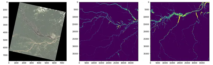
The first thing you may have noticed is that the arrays have different sizes. We can print the shapes to check:
print(rgb.shape, water1_array.shape, water2_array.shape)

code output:
(7761, 7601, 3) (40000, 40000) (40000, 40000)
So, how can we superpose and compare these arrays? First, we need to understand why they appear so different.
Step 2- Coordinate Reference Systems
When we load a satellite raster image into a Python array, it is just that, an array. We don’t have any information about the location on earth of these pixels. For this, two things are necessary:
A system (logic) to map earth locations into coordinates (Coordinate Reference System); and
Something to tell us where in this coordinate system lies our array (GeoTransformation).
A will give here a very brief introduction to CRSs to understand how to correctly manipulate our raster image, but there other good online resources if you want to go deeper in this subject.
Types of Coordinate Reference Systems
Coordinate reference systems, or spatial reference systems, describe how we can map the earth's surface into coordinates. There exists two main types:
Geographic Coordinate Systems: in GCS, the mathematical model tries to match the position on earth by approximating the earth to an ellipsoid (which one will depend on the Datum we are using). The coordinates are then measured in degrees (latitude and longitude). GCS are best for global analysis (Figure 2-a) however the distances (and areas) are distorted. For example, one degree of longitude around equator has a different distance from one degree on longitude near the poles;
Projected Coordinate Systems: the PCS represent the surface of the earth (or a portion of it) in a flat 2 dimensional coordinate system (for example a flat piece of paper or computer screen). It is necessary to use a map projection, to transform the earth from its spherical shape (3D) to a planar shape (2D). There are three main types of map projections that can be visualized in Figure 2-b (cylindrical, planar and conical). They have been conceived for different objectives: preserve angles, preserve areas, etc.

Although our recently loaded arrays don't have any geographic information, let's access the dataset loaded by rasterio. The profile attribute is a dictionary, and if we print it (bellow), we can se that one of the keys is "crs" (in bold). Note that the water occurrence masks have CRS = CRS.from_epsg(4326) and the landsat image has CRS = CRS.from_epsg(32620).
print('Image: \n', image_ds['B2'].profile)
print('Water mask 1: \n', water1_ds.profile)
print('Water mask 2: \n', water2_ds.profile)

Code output:
Image:
 {'driver': 'GTiff', 'dtype': 'uint16', 'nodata': 0.0, 'width': 7601, 'height': 7761, 'count': 1, 'crs': CRS.from_epsg(32620), 'transform': Affine(30.0, 0.0, 658185.0,
       0.0, -30.0, -203985.0), 'blockxsize': 256, 'blockysize': 256, 'tiled': True, 'compress': 'deflate', 'interleave': 'band'}

Water mask 1:
 {'driver': 'GTiff', 'dtype': 'uint8', 'nodata': None, 'width': 40000, 'height': 40000, 'count': 1, 'crs': CRS.from_epsg(4326), 'transform': Affine(0.00025, 0.0, -70.0,
       0.0, -0.00025, 0.0), 'blockxsize': 256, 'blockysize': 256, 'tiled': True, 'compress': 'lzw', 'interleave': 'band'}

Water mask 2:
 {'driver': 'GTiff', 'dtype': 'uint8', 'nodata': None, 'width': 40000, 'height': 40000, 'count': 1, 'crs': CRS.from_epsg(4326), 'transform': Affine(0.00025, 0.0, -60.0,
       0.0, -0.00025, 0.0), 'blockxsize': 256, 'blockysize': 256, 'tiled': True, 'compress': 'lzw', 'interleave': 'band'}
Note that we just have a code, called EPSG. EPSG is a public registry of coordinate systems and every one is assigned a unique number (the EPSG code).
Note: EPSG stands for European Petroleum Survey Group and is an organization that maintains a geodetic parameter database with standard codes, the EPSG codes (http://epsg.org) .
If we search the ESPG database (or google), for these EPSG codes, we can have the correct description each CRS we have.
EPSG 4326: WGS 84 Geographic
EPSG 32620: Projected UTM Zone 20N
GeoTransformation
Now that we know which are the CRSs of our images, we still need to understand how we can map the array indexes (rows and columns) to geographic coordinates of our CRS. The most common method is to consider our array to be a evenly spaced regular grid (each cell has the same size). In this case, we just have to know the correct location of one cell (the top left) and the cell dimensions (width and height) in the CRS units (degrees for the geographic CRS and meters for the UTM, for example). The mapping of array index (row, column) into CRSs coordinates is done by the GeoTransformation. This transformation is also stored in the dataset profile and if we apply it to any dataset position we receive the its corresponding CRS coordinate.
Let's try to apply the transformation of any band (B2, for example) to the first top-left cell (0, 0) and the bottom-right cell (width, height). To apply it, we can do use AffineMatrix * (column, row) and the results will be (x, y) in the CRSs units. Then, we can compare the result with the extents of the dataset and confirm that they match perfectly.
Code output:
(658185.0, -203985.0)
(886215.0, -436815.0)
BoundingBox(left=658185.0, bottom=-436815.0, right=886215.0, top=-203985.0)
Step 3- Re-projecting
Now that we know how a CRS works, its easy to understand why we cannot simply compare the pixels of our arrays. So, the first thing we have to do is to convert the arrays to the same CRS. As we will want to superpose the water mask into our Amazon image, we are going to convert the water masks from EPSG 4326 to EPSG 32620. To perform the reprojection we will use the reproject function defined in the warp module of the rasterio. We will pass as arguments, the source as a rasterio band object (that’s the reason for the rasterio.band applied to the dataset), the desired CRS, and the destination resolution.
Step 4- Merging
To make things a little more difficult here, our Landsat 8 image lies into two different water mask tiles, so we cannot just cut the portion we want. We will first merge the two water masks into one. This will be done by using the merge function from rasterio.merge module.
Note: The merge function requires two rasterio datasets, however we have the reprojected arrays (and transforms) instead. In this case, we have to write our reprojected results into new datasets. Instead of writing new datasets to file, we will use the rasterio.io.MemoryFile class to keep everything in memory.
We will define a create_dataset function that will receive the array, the CRS and the transformation to return a in-memory rasterio dataset. After we have our datasets, we will be able to call the merge function. At the end we will display the merged water mask.

The merging seems to have worked fine, but the question is: Where is our Area of Interest (Manaus region) here?
Step 5- Cropping
Now that we have a big, merged, water occurrence map in the same CRS as our Landsat 8 image, it is time to crop it using the extents of our Area of Interest. So, the first thing to do now is to get the extents of the Landsat image. We have seen in Step 2 that we can use the bounds method to get a dataset extents. However, the crop method from rasterio receives a GeoJSON as input to do the crop.
We can extract the GeoJSON of our landsat image do this using the rasterio.features.shapes function, that will return us a GeoJSON of the shapes it identifies in a given dataset. As we want the whole image, we can pass just an empty array with the same shape of the Landsat image. The trick here is that the shapes functions returns a “generator”, that permits us to iterate through the various results. We are not going into details of yield and generators here, but as we expect just one output (the polygon with the entire image) we are going to use the python’s built in next function, like so:
next(shapes(np.zeros_like(img['B2']), transform=image_ds['B2'].profile['transform']))

Results:
({'type': 'Polygon',
  'coordinates': [[(658185.0, -203985.0),
    (658185.0, -436815.0),
    (886215.0, -436815.0),
    (886215.0, -203985.0),
    (658185.0, -203985.0)]]},
 0.0)
Like before, the crop function requires a dataset as argument, so we will create the merged_ds beforehand. The, we will crop to the extents we just retrieved and display the results.

Step 6- Superposing the layers
New we can use the plot_masked_rgb function defined in part 4 to superpose the mask with the whole Landsat Image. A small adjustment is required in the cropped shape, as the rasterio’ s mask function returned additional pixel that can be discarded. As the occurrence water mask from the Global Surface Water is provided in a 0–100 scale (100 meaning 100% of occurrence of water over time) and we are expecting a TRUE/FALSE mask, we can use the logical operand greater than to get the pixels with more than 80% of water: mask = cropped[0]>80. Additionally, we will ignore the pixels that have no value in the Landsat image, trhough the command mask = np.where(img[‘B2’] == 0, 0, mask) and plot our supperposed image, as usual.

Notebook
As always, here is the notebook with all the code needed to run these examples.
Conclusion
Today we overviewed some important concepts about geospatial data, like Coordinate Reference Systems and GeoTransforms and how to move from one system to another using the rasterio package. The tasks of reprojecting, clipping and merging are usually necessary when we need to compare data that is saved in different projection systems. They can be done using GIS software such as QGIS or ESRI’s ArcGIS, but with Python it is possible to write a chain to automate these steps.
Hope you have enjoyed, stay tuned and see you next story!
Previous Posts
Link for the previous posts of Python for Geosciences series:
Part 1 - Working with Satellite Images
Part 2- Satellite Image Analysis
Part 3- Spectral Analysis
Part 4- Raster bit masks explained
Part 5- Raster Merging, Clipping and Reprojection with Rasterio
Part 6- Scatter plots and PDF Reports
References:
[1] Pekel, J.-F.; Cottam, A.; Gorelick, N.; Belward, A. S. High-Resolution Mapping of Global Surface Water and Its Long-Term Changes. Nature 2016, 540 (7633), 418–422. https://doi.org/10.1038/nature20584.
Comments